Iraq War Logs Dataset data manipulation with Dask

Introduction

The main idea of this post is to filter, clean and prepare a portion of the Iraq War Logs Dataset in order to create a data visualization.

I wanted to create a new dichotomous variable to classify the attacks and incidents into two categories: those that happened at daylight and those that occurred at nighttime.

Using Pandas’ apply function would take forever, so I will use Dask’s multiprocessing apply instead.

Requeriments

Filter by Indirect Fire, IED Explosions and Safire events.
Convert coordinates from MGRS coordinates to Lat Lon with WGS84 Datum.
Calculate Sunrise and Sunset local time from each event.
Create a new binary column indicating if the events occurred between Sunrise and Sunset.

Libraries

Script

The cript has three main parts:

Data filtering and formatting.
Coordinates conversion.
Sunset/Sunrise calculations.

Data preparation

Our subset of Iraq War Logs dataset will contain all the IDF, IED and Safire events where Coalition Forces or the Iraqi Security Forces were involved.

To properly manipulate the Datetime column, it will be converted to a Pandas datetime type, and we will map the Type of unit column to normalize the labels.

def dataframe_format(iraq_dataset):
    """
    Data preprocessing. Filters the iraq_sigacts dataset by category (Indirect fire, IED and Safire) and by type of unit
    (CF, Coalition Forces and ISF).
    Converts Datetime column to datetime object with '%Y-%m-%d %H:%M' format and maps type of unit column to contain
    only Coalition forces and Iraqi Security Forces.
    Capitalizes Type, Category and Affiliation columns.
    :param iraq_dataset: iraq_sigacts dataset
    :return: Dataframe
    """
    # Read dsv data
    df = pd.read_csv(iraq_dataset).dropna()
    # Filter by IDF, IED and Safire
    df = df[df['Category'].str.contains('Indirect Fire|IED Explosion|Safire')]
    # Filter by CF and ISF
    df = df[df['Type_of_unit'].str.contains('CF|Coalition|Coalition Forces|ISF')]
    # Datetime format
    df['Datetime'] = pd.to_datetime(df['Datetime'])
    # Type of unit name normalization
    type_of_unit = {'CF': 'Coalition Forces',
                    'Coalition': 'Coalition Forces',
                    'ISF': 'Iraqi Security Forces'}
    df[df.columns] = df.applymap(lambda x: x.strip() if isinstance(x, str) else x)
    df["Type_of_unit"] = df['Type_of_unit'].map(type_of_unit).fillna(df['Type_of_unit'])
    # Capitalize string columns
    df[['Type', 'Category', 'Affiliation']] = df[['Type',
                                                  'Category',
                                                  'Affiliation']].apply(lambda x: x.str.capitalize())
    return df

After the data filtering we get a dataframe with 44,464 rows.

Coordinates conversion

Converting from MGRS to WGS84 is crucial for interactive maps due to compatibility and usability. MGRS, used in military operations, is not widely supported in most mapping software, whereas WGS84 is the global standard for coordinates, universally recognized by major GIS and mapping platforms.

def mgrs_to_latlon(x):
    """
    Converts MGRS coordinates to lat, lon format
    :param x: MGRS coordinates
    :return: Lat, Lon coordinates
    """
    try:
        # Initialize MGRS object
        m = mgrs.MGRS()
        latlon = m.toLatLon(x)
        lat, lon = latlon
        lat = str(lat).replace("(","")
        lon = str(lon).replace(")","")
        return float(lat), float(lon)
    except Exception:
        return np.nan, np.nan

Sunrise, sunset and daytime computations

We are computing sunset, sunrise, and daytime for specific locations and dates using Dask for parallel processing. The function sun calculates the local times for sunset and sunrise, as well as a binary daylight indicator, by leveraging ephemeris data to determine the sun’s position. Each row in the DataFrame, which includes latitude, longitude, and datetime columns, is processed row-wise in parallel using Dask.

This approach efficiently handles large datasets, enabling rapid computation of these solar events across many records simultaneously. The resulting times are adjusted to the local timezone, ensuring accurate and relevant data for each location.

def sun(df):
    """
    Calculates the sunset and sunrise (local time) for a specific location (lat, lon) and a specific day.
    Creates a dichotomous variable called daylight with 1 if the event occurred at daylight.
    :param df: Dataframe that contains lat, lon and Datetime column.
    :return:
    sunset with format %Y-%m-%dT%H:%M:%S
    sunrise with format %Y-%m-%dT%H:%M:%S
    daylight dichotomous variable.
    """
    try:
        # Ephemeris bsp file to calculate the position of the sun at a specific location and date.
        eph = api.load('de421.bsp')
        ts = api.load.timescale()
        # GeographicPosition object
        location = api.wgs84.latlon(df['lat'], df['lon'])
        # Two UTC timescale object to find sunsets sunrise in between
        t0 = ts.utc(df['Datetime'].year, df['Datetime'].month, df['Datetime'].day, 0)
        t1 = ts.utc(df['Datetime'].year, df['Datetime'].month, df['Datetime'].day, 23)
        # Find all sunsets and sunrises at location between t0 and t1
        t, y = almanac.find_discrete(t0, t1, almanac.sunrise_sunset(eph, location))
        # Sunrise and sunset with UTC +3 (Iraq Offset)
        sunrise = datetime.strptime(t.utc_iso()[0], '%Y-%m-%dT%H:%M:%SZ') + timedelta(hours=3)
        sunset = datetime.strptime(t.utc_iso()[1], '%Y-%m-%dT%H:%M:%SZ') + timedelta(hours=3)
        # Conditional if the event is at daylight ot not
        if sunrise.time() < df['Datetime'].time() < sunset.time():
            daylight = 1
            return sunrise, sunset, daylight
        else:
            daylight = 0
            return sunrise, sunset, daylight
    except Exception:
        return np.nan, np.nan, np.nan

Dask parallel compute vs Pandas apply

We are setting up a Dask client with 6 workers and splitting the dataset into 500 partitions for parallel processing. The sun function is applied row-wise to each partition, and the results are specified to include ‘Sunrise’ and ‘Sunset’ as datetime columns, and ‘Daylight’ as an integer column.

The computation is executed with Dask’s process-based scheduler, ensuring efficient parallel execution. After processing, the Dask client is shut down.

 # Dask Client with 6 workers
client = Client(n_workers=6)

# Convert df to a Dask dataframe with 500 partitions
ddata = dd.from_pandas(df,
                       npartitions=500)

start_time = time.time()
print('Executing Dask with 6 workers and 12 threads')
with ProgressBar():
    # Apply sun function with dask parallel processing and compute the dask object to get a pandas df.
    df[['Sunrise', 'Sunset', 'Daylight']] = ddata.apply(f.sun,
                                                        axis=1,
                                                        result_type="expand",
                                                        meta={0: 'datetime64[ns]',
                                                              1: 'datetime64[ns]',
                                                              2: 'int64'}).compute(scheduler='processes')

client.shutdown()

Parallel animation

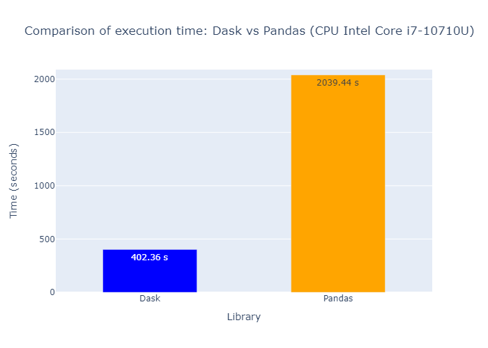
Performance comparison

To compare the performance of the two approaches, we measure the time taken to compute the sunrise, sunset, and daylight columns for the “War Diary: Iraq War Logs” dataset, which contains 44,464 entries. Using an Intel Core i7-10710U CPU with 6 cores, it took:

Dask multiprocess time: 402.36 seconds
Pandas apply time: 2039.44 seconds

Comparison chart

About me

My name is Martin, and I am a Data Scientist.

Repository link on Github